Skip over navigation
Article by Michael Grayling
Many students have an aversion to Statistics questions when it comes to STEP, most probably because it is often given a somewhat peripheral role in many A-Level specifications in comparison to topics such as differentiation. However, in actuality the questions can often be very nice; frequently only revolving around a few key concepts and some basic skills with algebra and integration. Thus, there is no reason to fear such questions even if you haven't completed many A-Level Statistics modules. Here we will quickly go over the core techniques that you will need to master to maximise your chances when it comes to attempting STEP Statistics questions, before going through some examples. Our focus specifically will be on the standard discrete and continuous random variables; how we compute expectations and variances. The issue of hypothesis testing, also key to Statistics, is discussed here. With statistics so intrinsically linked to Probability, it will also almost certainly assist you to go over Module 16 as well which covers more closely computing probabilities in non-standard situations!
Discrete and Continuous Random Variables
The first thing you will need to ensure before approaching a STEP Statistics question is that you have got to grips with all of the most common discrete and continuous random variables. To jog your memory, a random variable is simply a variable which takes on one of a set of values due to chance.
So, we begin with discrete random variables. Suppose that this random variable is called \(X\). Then, here, \(X\) can only take on one of a particular enumerable list of values, and we have what is known as a probability mass function (PMF). This tells us the probability each of these values is taken on by the random variable, i.e. the value of \( \mathbb{P}(X=x) \). Additionally, its common to denote the cumulative distribution function (CDF) by \( F(x) = \mathbb{P}(X \leq x) \). Armed with these functions, there are then several key formulae to recall: describing a property of the PMF, what value we expect the random variable to take, and how much we expect the value of the random variable to vary by respectively:
\( \hspace{0.5 in} \sum_{\forall x} \mathbb{P}(X=x) = 1, \hspace{0.2 in} \mathbb{E}(X) = \sum_{\forall x} x\mathbb{P}(X=x), \hspace{0.2 in} Var(X) = \mathbb{E}(X^2) - \mathbb{E}(X)^2. \)
Amazingly, the above actually encompasses the majority of what you need to know about discrete random variables; when faced with a difficult question it is almost certainly worthwhile trying to make progress simply with these formulae first. However, we must also focus in slightly more detail on two example discrete distributions.
The Binomial distribution describes the distribution of the number of successes in a sequence of n independent experiments, each yielding a yes/no answer with probability \(p\). Here, the distribution is completely characterised by the values of \(n\) and \(p\), so we tend to write \( X \sim Bin(n,p) \) and then we have:
\( \hspace{1 in} \mathbb{P}(X=x) = {n \choose x} p^x (1-p)^{n-x}, \hspace{0.2 in} \mathbb{E}(X) = np, \hspace{0.2 in} Var(X) = np(1-p). \)
The Poisson distribution describes the probability of a number of events occurring in a fixed interval of time or space, if these events occur with a known average rate. Then, the distribution is completely characterised by the value of λ; the known average rate the events of interest occur at. We write \( X \sim Po(\lambda) \) and have:
\( \hspace{1.75 in} \mathbb{P}(X=x) = \frac{\lambda^xe^{-\lambda}}{x!}, \hspace{0.2 in} \mathbb{E}(X) = \lambda, \hspace{0.2 in} Var(X) = \lambda. \)
OK, so that's all on discrete random variables, but what about continuous? Well, let's suppose we have a continuous random variable \(Y\), then we can no longer write down the probability \(Y\) takes on every value it potentially can; there would simply be too many (infinitely many!). Moreover, how would we define the probability of taking exactly a particular height for example: how accurately can we measure? Instead, we have a probability density function (PDF) \(f(y)\) which allows us to compute the probability \(Y\) lies in a particular range using integration:
\( \hspace{2.8 in} \mathbb{P}(a < Y < b) = \int_{a}^{b} f(y)dy. \)
Analogously to the discrete case, our key formulae are then:
\( \hspace{0.15 in} \int_{\forall y}f(y)dy = 1, \hspace{0.2 in} F(y)=\mathbb{P}(Y \leq y), \hspace{0.2 in} \mathbb{E}(Y)=\int_{\forall y}yf(y)dy, \hspace{0.2 in} Var(Y) = \mathbb{E}(Y^2) - \mathbb{E}(Y)^2. \)
So that's the basics we need to know. However, there are again particular distributions for which we should recall more.
The uniform, or continuous rectangular, distribution is such that all intervals of the same length on its possible range of values are equally probable. So, all we need to know is the end points of the range of values it can take, and we write \(Y \sim U(a,b) \) implying:
\( \hspace{1.4 in} f(y)=\frac{1}{b-a}, \hspace {0.2 in} \mathbb{E}(Y)=\frac{1}{2}(a+b), \hspace{0.2 in} Var(Y)=\frac{1}{12} (b-a)^2. \)
The normal distribution is extremely important as it describes how many real variables work; the random variable is distributed evenly with some variance about some mean value. We write \( Y \sim N(\mu,\sigma^2) \) and have:
\( \hspace{1.7 in} f(y) = \frac{1}{\sigma \sqrt{2 \pi}} e^{-\frac{(y - \mu)^2}{2 \sigma^2}}, \hspace{0.2 in} \mathbb{E}(Y)=\mu, \hspace{0.2 in} Var(Y)=\sigma^2. \)
Since the normal distribution is so important, we also tend to give it special notation. We use \(Z\) instead of \(Y\), write its PDF as \( \phi(z) \), and set \( \Phi (z) = \mathbb{P}(Z \leq z) \). Then, the symmetric nature of the normal distribution also gives us \( \Phi (z) = 1 - \Phi (-z) \).
So we've now covered all of the crucial ideas behind continuous and discrete random variables; it therefore makes sense to go through an example!

Now this is a really useful question to illustrate some of the points made above. For the most part, all we are going to use is those basic formulae on continuous random variables: which means all you really need to be able to solve this question is a knowledge of integration!
\( \hspace{3 in} \int_{-\infty}^{\infty}f(x)dx=1. \)
$$ \eqalign{ \int_{-\infty}^{\infty}f(x)dx=1\Rightarrow k\left [ \int_{-\infty}^{\infty}\phi(x)dx + \lambda\int_{0}^{\lambda}g(x)dx\right ]&=1,
\cr \Rightarrow k\left [ 1 + \lambda\int_{0}^{\lambda}\frac{1}{\lambda}dx\right ]&=1,
\cr \Rightarrow k\left \{ 1+\lambda\left [ \frac{x}{\lambda} \right ]^{\lambda}_0 \right \}&=1,
\cr \Rightarrow k(1+\lambda)&=1,
\cr \Rightarrow k&=\frac{1}{1+\lambda}.} $$
\( \mu=\mathbb{E}(X)=\int^{\infty}_{-\infty}xf(x)dx=k\int^{\infty}_{-\infty}x\phi(x)dx+\int^{\lambda}_{0}\frac{x}{\lambda}dx=0+k\lambda\left [ \frac{x^2}{2\lambda} \right ]^{\lambda}_0=\frac{1}{2}k\lambda^2=\frac{\lambda^2}{2(1+\lambda)}.\)
Here we have made use of the fact that the normal part has mean 0.
So what about the standard deviation? Well, as noted earlier, most of the time it's best just to use the formula \( \sigma^2 = Var(X) = \mathbb{E}(X^2) - \mathbb{E}(X)^2 \). To do so, we first compute \(\mathbb{E}(X^2)\):
\( \hspace{2 in} \eqalign{ \mathbb{E}(X^2)&=\int^{\infty}_{-\infty}x^2f(x)dx, \cr &= k\int^{\infty}_{-\infty}x^2\phi(x)dx+k\lambda\int^{\lambda}_0\frac{x^2}{\lambda}dx, \cr &=k+k\lambda\left [ \frac{x^3}{3\lambda} \right ]^{\lambda}_0, \cr &= k+\frac{k\lambda^3}{3}, \cr &= k\left ( 1+\frac{\lambda^3}{3} \right ).} \)
Thus, we then have:
\( \hspace{1.7 in} \sigma^2=Var(X)=\frac{3+\lambda^3}{3(1+\lambda)}-\left [ \frac{\lambda^2}{2(1+\lambda)} \right ]^2=\frac{\lambda^4+4\lambda^3+12\lambda+12}{12(1+\lambda)^2},\)
as required.
For the next part, we first note that if \(\lambda=2\) then:
\( \hspace{2 in} k=1/3,\hspace{0.2 in} \mu=2/3, \hspace{0.2 in} \sigma^2=\frac{16+32+24+12}{108}=\frac{7}{9}.\)
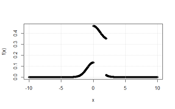
So now \( f(x)=1/3 [\phi(x)+2g(x)]\) and \(g(x)=1/2\) for \(0\leq x\leq2\). Therefore the graph is simply the standard normal curve \(y=1/3 \phi(x)\) with the portion from \(x=0\) to \(x=2\) lifted vertically through a distance of \(1/3\), i.e.:

(iii) We can use the graph above, with a little help from the PDF to see that \(F(x)\) is given by:
\( \hspace{2.4 in} F(x)=\left\{\begin{matrix}
\frac{1}{3}\Phi(x):x\leq0,\\
\frac{1}{3}\Phi(x)+\frac{x}{3}:0\leq x\leq2,\\
\frac{1}{3}\Phi(x)+\frac{2}{3}:2\leq x.\\
\end{matrix}\right. \)
i.e. we simply have one third of the standard normal CDF across \(x\), but must factor in the CDF corresponding to \(g\) for \(x \geq 0\).
Finally, we can use the above CDF to quickly compute the required probability. We have:
\( \hspace{1 in} \eqalign{ \mathbb{P}\left(0 < X < \frac{2}{3}+\frac{2}{3}\sqrt{7}\right)&=\frac{1}{3}\Phi(\frac{2}{3}+\frac{2}{3}\sqrt{7})+\frac{2}{3}-\frac{1}{3}\Phi(0), \cr &= \frac{0.9921}{3}+0.6667-\frac{0.5}{3}, \cr &=0.8307. } \)
where the only final step here was to realise that \( 2/3+2/3\sqrt{7} > 2 \).
OK, so that completes the question! Hopefully, you should be relatively convinced that all we needed was a knowledge of how continuous random variables work, and some basic integration skills: nothing to fear even for those who haven't got much experience in Statistics.
Or search by topic
Number and algebra
Geometry and measure
Probability and statistics
Working mathematically
Advanced mathematics
For younger learners
Age 16 to 18
Published 2014 Revised 2017
Statistics in Exams: Discrete and Continuous Random Variables
Why Statistics?
Many students have an aversion to Statistics questions when it comes to STEP, most probably because it is often given a somewhat peripheral role in many A-Level specifications in comparison to topics such as differentiation. However, in actuality the questions can often be very nice; frequently only revolving around a few key concepts and some basic skills with algebra and integration. Thus, there is no reason to fear such questions even if you haven't completed many A-Level Statistics modules. Here we will quickly go over the core techniques that you will need to master to maximise your chances when it comes to attempting STEP Statistics questions, before going through some examples. Our focus specifically will be on the standard discrete and continuous random variables; how we compute expectations and variances. The issue of hypothesis testing, also key to Statistics, is discussed here. With statistics so intrinsically linked to Probability, it will also almost certainly assist you to go over Module 16 as well which covers more closely computing probabilities in non-standard situations!
Discrete and Continuous Random Variables
The first thing you will need to ensure before approaching a STEP Statistics question is that you have got to grips with all of the most common discrete and continuous random variables. To jog your memory, a random variable is simply a variable which takes on one of a set of values due to chance.
So, we begin with discrete random variables. Suppose that this random variable is called \(X\). Then, here, \(X\) can only take on one of a particular enumerable list of values, and we have what is known as a probability mass function (PMF). This tells us the probability each of these values is taken on by the random variable, i.e. the value of \( \mathbb{P}(X=x) \). Additionally, its common to denote the cumulative distribution function (CDF) by \( F(x) = \mathbb{P}(X \leq x) \). Armed with these functions, there are then several key formulae to recall: describing a property of the PMF, what value we expect the random variable to take, and how much we expect the value of the random variable to vary by respectively:
\( \hspace{0.5 in} \sum_{\forall x} \mathbb{P}(X=x) = 1, \hspace{0.2 in} \mathbb{E}(X) = \sum_{\forall x} x\mathbb{P}(X=x), \hspace{0.2 in} Var(X) = \mathbb{E}(X^2) - \mathbb{E}(X)^2. \)
Amazingly, the above actually encompasses the majority of what you need to know about discrete random variables; when faced with a difficult question it is almost certainly worthwhile trying to make progress simply with these formulae first. However, we must also focus in slightly more detail on two example discrete distributions.
The Binomial distribution describes the distribution of the number of successes in a sequence of n independent experiments, each yielding a yes/no answer with probability \(p\). Here, the distribution is completely characterised by the values of \(n\) and \(p\), so we tend to write \( X \sim Bin(n,p) \) and then we have:
\( \hspace{1 in} \mathbb{P}(X=x) = {n \choose x} p^x (1-p)^{n-x}, \hspace{0.2 in} \mathbb{E}(X) = np, \hspace{0.2 in} Var(X) = np(1-p). \)
The Poisson distribution describes the probability of a number of events occurring in a fixed interval of time or space, if these events occur with a known average rate. Then, the distribution is completely characterised by the value of λ; the known average rate the events of interest occur at. We write \( X \sim Po(\lambda) \) and have:
\( \hspace{1.75 in} \mathbb{P}(X=x) = \frac{\lambda^xe^{-\lambda}}{x!}, \hspace{0.2 in} \mathbb{E}(X) = \lambda, \hspace{0.2 in} Var(X) = \lambda. \)
OK, so that's all on discrete random variables, but what about continuous? Well, let's suppose we have a continuous random variable \(Y\), then we can no longer write down the probability \(Y\) takes on every value it potentially can; there would simply be too many (infinitely many!). Moreover, how would we define the probability of taking exactly a particular height for example: how accurately can we measure? Instead, we have a probability density function (PDF) \(f(y)\) which allows us to compute the probability \(Y\) lies in a particular range using integration:
\( \hspace{2.8 in} \mathbb{P}(a < Y < b) = \int_{a}^{b} f(y)dy. \)
Analogously to the discrete case, our key formulae are then:
\( \hspace{0.15 in} \int_{\forall y}f(y)dy = 1, \hspace{0.2 in} F(y)=\mathbb{P}(Y \leq y), \hspace{0.2 in} \mathbb{E}(Y)=\int_{\forall y}yf(y)dy, \hspace{0.2 in} Var(Y) = \mathbb{E}(Y^2) - \mathbb{E}(Y)^2. \)
So that's the basics we need to know. However, there are again particular distributions for which we should recall more.
The uniform, or continuous rectangular, distribution is such that all intervals of the same length on its possible range of values are equally probable. So, all we need to know is the end points of the range of values it can take, and we write \(Y \sim U(a,b) \) implying:
\( \hspace{1.4 in} f(y)=\frac{1}{b-a}, \hspace {0.2 in} \mathbb{E}(Y)=\frac{1}{2}(a+b), \hspace{0.2 in} Var(Y)=\frac{1}{12} (b-a)^2. \)
The normal distribution is extremely important as it describes how many real variables work; the random variable is distributed evenly with some variance about some mean value. We write \( Y \sim N(\mu,\sigma^2) \) and have:
\( \hspace{1.7 in} f(y) = \frac{1}{\sigma \sqrt{2 \pi}} e^{-\frac{(y - \mu)^2}{2 \sigma^2}}, \hspace{0.2 in} \mathbb{E}(Y)=\mu, \hspace{0.2 in} Var(Y)=\sigma^2. \)
Since the normal distribution is so important, we also tend to give it special notation. We use \(Z\) instead of \(Y\), write its PDF as \( \phi(z) \), and set \( \Phi (z) = \mathbb{P}(Z \leq z) \). Then, the symmetric nature of the normal distribution also gives us \( \Phi (z) = 1 - \Phi (-z) \).
So we've now covered all of the crucial ideas behind continuous and discrete random variables; it therefore makes sense to go through an example!
Example
2005 Paper II Question 14
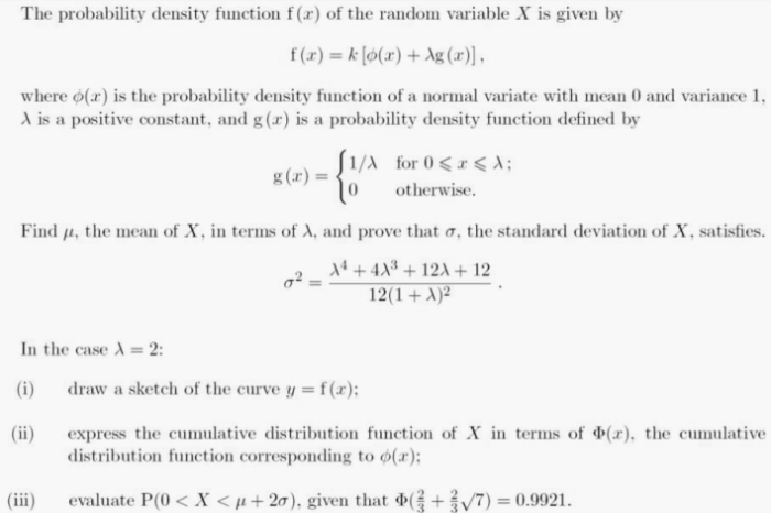
Now this is a really useful question to illustrate some of the points made above. For the most part, all we are going to use is those basic formulae on continuous random variables: which means all you really need to be able to solve this question is a knowledge of integration!
We begin by noticing that it wants our mean \(\mu\) in terms of \(\lambda\), but we have an unknown \(k\) in our PDF. Fortunately for us, we can recall that this PDF must satisfy:
\( \hspace{3 in} \int_{-\infty}^{\infty}f(x)dx=1. \)
Here, the limits are from positive to negative \(\infty\) because the normal part of the PDF is defined for all real \(x\). So what does the above imply:
$$ \eqalign{ \int_{-\infty}^{\infty}f(x)dx=1\Rightarrow k\left [ \int_{-\infty}^{\infty}\phi(x)dx + \lambda\int_{0}^{\lambda}g(x)dx\right ]&=1,
\cr \Rightarrow k\left [ 1 + \lambda\int_{0}^{\lambda}\frac{1}{\lambda}dx\right ]&=1,
\cr \Rightarrow k\left \{ 1+\lambda\left [ \frac{x}{\lambda} \right ]^{\lambda}_0 \right \}&=1,
\cr \Rightarrow k(1+\lambda)&=1,
\cr \Rightarrow k&=\frac{1}{1+\lambda}.} $$
Brilliant; we have a formulae for \(k\) in terms of \(\lambda\)! This means if we simply look to compute the mean \(\mu\) then we can replace any unwanted \(k\)'s for \(\lambda\)'s:
\( \mu=\mathbb{E}(X)=\int^{\infty}_{-\infty}xf(x)dx=k\int^{\infty}_{-\infty}x\phi(x)dx+\int^{\lambda}_{0}\frac{x}{\lambda}dx=0+k\lambda\left [ \frac{x^2}{2\lambda} \right ]^{\lambda}_0=\frac{1}{2}k\lambda^2=\frac{\lambda^2}{2(1+\lambda)}.\)
Here we have made use of the fact that the normal part has mean 0.
So what about the standard deviation? Well, as noted earlier, most of the time it's best just to use the formula \( \sigma^2 = Var(X) = \mathbb{E}(X^2) - \mathbb{E}(X)^2 \). To do so, we first compute \(\mathbb{E}(X^2)\):
\( \hspace{2 in} \eqalign{ \mathbb{E}(X^2)&=\int^{\infty}_{-\infty}x^2f(x)dx, \cr &= k\int^{\infty}_{-\infty}x^2\phi(x)dx+k\lambda\int^{\lambda}_0\frac{x^2}{\lambda}dx, \cr &=k+k\lambda\left [ \frac{x^3}{3\lambda} \right ]^{\lambda}_0, \cr &= k+\frac{k\lambda^3}{3}, \cr &= k\left ( 1+\frac{\lambda^3}{3} \right ).} \)
Thus, we then have:
\( \hspace{1.7 in} \sigma^2=Var(X)=\frac{3+\lambda^3}{3(1+\lambda)}-\left [ \frac{\lambda^2}{2(1+\lambda)} \right ]^2=\frac{\lambda^4+4\lambda^3+12\lambda+12}{12(1+\lambda)^2},\)
as required.
For the next part, we first note that if \(\lambda=2\) then:
\( \hspace{2 in} k=1/3,\hspace{0.2 in} \mu=2/3, \hspace{0.2 in} \sigma^2=\frac{16+32+24+12}{108}=\frac{7}{9}.\)
So now \( f(x)=1/3 [\phi(x)+2g(x)]\) and \(g(x)=1/2\) for \(0\leq x\leq2\). Therefore the graph is simply the standard normal curve \(y=1/3 \phi(x)\) with the portion from \(x=0\) to \(x=2\) lifted vertically through a distance of \(1/3\), i.e.:

(iii) We can use the graph above, with a little help from the PDF to see that \(F(x)\) is given by:
\( \hspace{2.4 in} F(x)=\left\{\begin{matrix}
\frac{1}{3}\Phi(x):x\leq0,\\
\frac{1}{3}\Phi(x)+\frac{x}{3}:0\leq x\leq2,\\
\frac{1}{3}\Phi(x)+\frac{2}{3}:2\leq x.\\
\end{matrix}\right. \)
i.e. we simply have one third of the standard normal CDF across \(x\), but must factor in the CDF corresponding to \(g\) for \(x \geq 0\).
Finally, we can use the above CDF to quickly compute the required probability. We have:
\( \hspace{1 in} \eqalign{ \mathbb{P}\left(0 < X < \frac{2}{3}+\frac{2}{3}\sqrt{7}\right)&=\frac{1}{3}\Phi(\frac{2}{3}+\frac{2}{3}\sqrt{7})+\frac{2}{3}-\frac{1}{3}\Phi(0), \cr &= \frac{0.9921}{3}+0.6667-\frac{0.5}{3}, \cr &=0.8307. } \)
where the only final step here was to realise that \( 2/3+2/3\sqrt{7} > 2 \).
OK, so that completes the question! Hopefully, you should be relatively convinced that all we needed was a knowledge of how continuous random variables work, and some basic integration skills: nothing to fear even for those who haven't got much experience in Statistics.

