Skip over navigation


We were sent two very impressive solutions to this fascinating problem. We can only assume that Ben from Kenny and Paul (no location given) are going to go on to do great things mathematically!
Both solutions were formatted in careful detail, so we include the two pdf files directly for Paul and Ben. Ben also included his geogebra file for you to have a look at.
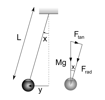
No radial acceleration as $F_{rad}$ balanced by tension in string.
Newton's Second Law:
$$\sum_{i}\mathbf{F_i} = \frac{\textrm{d}}{\textrm{d}t}(m \mathbf{v})\;.$$
Considering the tangential direction:
$$F_{tan} = mg \sin x \quad\textrm{ and }\quad a_{tan} = -\ddot{x} \ell $$
$$\Rightarrow -mg \sin x = m\ddot{x}\ell\;.$$
$\sin x = \frac{y}{\ell}$ from trigonometric definitions $\Rightarrow y = \ell \sin x\;.$
For small $x$ ($x < 20^\circ$ from question), $\sin x \approx x$
$$\Rightarrow y = \ell x \Rightarrow \ddot{x} = \frac{\ddot{y}}{\ell}\;.$$
Substituting:
$$
\begin{align}
mg \frac{y}{\ell} &= -m \frac{\ddot{y}}{\ell} \ell\\
\frac{mg}{\ell}y &= -m\ddot{y}\\
m\ddot{y} + \frac{mg}{l}y &= 0
\end{align}
$$
$\Rightarrow k = \sqrt{\frac{mg}{\ell}}$ with units $\sqrt{\textrm{kg}}\ \textrm{s}^{-1}\;.$
$$
\begin{align}
y &= \exp \left[ \frac{-\lambda}{2m} t \right] \left( C \left[ \cos (\Lambda t) + i \sin (\Lambda t) \right] + D \left[ \cos (\Lambda t) - i \sin (\Lambda t) \right] \right)\;,\\
y &= \exp \left[ \frac{-\lambda}{2m} t \right] \left[ (C+D) \cos (\Lambda t) + i(C-D) \sin (\Lambda t) \right]\;.
\end{align}
$$
Let $A = C + D$ and $B = i(C-D)$:
$$y = \exp \left[ \frac{-\lambda}{2m} t \right] \left[ A \cos (\Lambda t) +B \sin (\Lambda t) \right]\;.$$
Therefore,
$$
\begin{align}
\dot{y} &= \frac{-\lambda}{2m} \exp \left[ \frac{-\lambda}{2m} t \right] \left[ A \cos (\Lambda t)+B \sin(\Lambda t) \right] + \exp \left[ \frac{-\lambda}{2m} t \right]\left[ - \Lambda A \sin (\Lambda t) + \Lambda B \cos (\Lambda t) \right]\\
\dot{y} &= \exp \left[ \frac{-\lambda}{2m} t \right] \left[ \left(\Lambda B - \frac{\lambda}{2m}A \right) \cos (\Lambda t) - \left(\Lambda A + \frac{\lambda}{2m}B \right) \sin (\Lambda t) \right]
\end{align}
$$
and
$$
\begin{align}
\ddot{y} &= \frac{-\lambda}{2m} \exp \left[ \left(\Lambda B - \frac{\lambda}{2m}A \right) \cos (\Lambda t) - \left(\Lambda A + \frac{\lambda}{2m}B \right) \sin (\Lambda t) \right] + \\
& \qquad \exp \left[ \frac{-\lambda}{2m} t \right] \left[ -\Lambda \left(\Lambda B - \frac{\lambda}{2m}A \right) \sin (\Lambda t) - \Lambda \left(\Lambda A + \frac{\lambda}{2m}B \right) \cos (\Lambda t) \right]\\
\ddot{y} &= \exp\left[ \frac{-\lambda}{2m} t \right] \left[ \left( \left( \frac{\lambda}{2m} \right)^2 A - 2 \left( \frac{\lambda}{2m} \right) B - \Lambda^2 A \right) \cos (\Lambda t)\right. + \\
& \qquad\left.\left( \left( \frac{\lambda}{2m} \right)^2 B + 2 \left( \frac{\lambda}{2m} \right) A - \Lambda^2 B \right) \sin (\Lambda t) \right]
\end{align}
$$
Substituting back in to $ m\ddot{y} + \lambda \dot{y} + k^2 y = 0$ gives:
$$
\begin{align}
0 =
& m \left\{
\exp \left[ \frac{-\lambda}{2m} t \right] \left[ \left( \left( \frac{\lambda}{2m} \right)^2 A - 2 \left( \frac{\lambda}{2m} \right) B - \Lambda^2 A \right) \cos (\Lambda t) + \right.\right.\\
&\qquad\left.\left.\left( \left( \frac{\lambda}{2m} \right)^2 B + 2 \left( \frac{\lambda}{2m} \right) A - \Lambda^2 B \right) \sin (\Lambda t) \right]
\right\} + \\
& \qquad\lambda \left\{
\exp \left[ \frac{-\lambda}{2m} t \right] \left[ \left(\Lambda B - \frac{\lambda}{2m}A \right) \cos (\Lambda t) - \left(\Lambda A + \frac{\lambda}{2m}B \right) \sin (\Lambda t) \right]
\right\} + \\
& \qquad k^2 \left\{
\exp \left[ \frac{-\lambda}{2m} t \right] \left[ A \cos (\Lambda t) +B \sin (\Lambda t) \right]
\right\}
\end{align}
$$
$$
\begin{align}
0 = \exp \left[ \frac{-\lambda}{2m} t \right]
& \cos (\Lambda t)
\left\{
m \left(\frac{\lambda}{2m}\right)^2 A - 2m \left(\frac{\lambda}{2m}\right) \Lambda B - m \Lambda^2 A + \right.\\
&\qquad\qquad\left.\lambda \Lambda B -\lambda \left(\frac{\lambda}{2m}\right) A + k^2 A
\right\} +
\\
& \sin (\Lambda t)
\left\{
m \left(\frac{\lambda}{2m}\right)^2 B + 2m \left(\frac{\lambda}{2m}\right) \Lambda A - m \Lambda^2 B - \right.\\
&\qquad\qquad\left.\lambda \Lambda A -\lambda \left(\frac{\lambda}{2m}\right) B + k^2 B
\right\}
\end{align}
$$
$$
\begin{align}
0 = \exp \left[ \frac{-\lambda}{2m} t \right]
& \cos (\Lambda t)
\left\{
\left(\frac{\lambda^2}{4m}\right) A - \lambda \Lambda B - m \left( \frac{k^2}{m}-\frac{\lambda^2}{4m^2} \right) A + \right.\\
&\qquad\qquad\left.\lambda \Lambda B -\left(\frac{\lambda^2}{2m}\right) A + k^2 A
\right\} +
\\
& \sin (\Lambda t)
\left\{
\left(\frac{\lambda^2}{4m}\right) B + \lambda \Lambda A - m \left( \frac{k^2}{m}-\frac{\lambda^2}{4m^2} \right) B - \right.\\
&\qquad\qquad\left.\lambda \Lambda A - \left(\frac{\lambda^2}{2m}\right) B + k^2 B
\right\}
\end{align}
$$
$$ \begin{align}
0 = \exp \left[ \frac{-\lambda}{2m} t \right]
& \cos (\Lambda t)
\left\{
\left(\frac{\lambda^2}{4m}\right) A - k^2 A + \left( \frac{\lambda^2}{4m} \right) A -\left(\frac{\lambda^2}{2m}\right) A + k^2 A
\right\} +
\\
& \sin (\Lambda t)
\left\{
\left(\frac{\lambda^2}{4m}\right) B - k^2 B + \left(\frac{\lambda^2}{4m} \right)B - \left(\frac{\lambda^2}{2m}\right) B + k^2 B
\right\}
\end{align}
$$
$$ 0= \exp \left[ \frac{-\lambda}{2m} t \right]
\cos (\Lambda t) \left\{ \left(\frac{\lambda^2}{2m}\right) A - \left(\frac{\lambda^2}{2m}\right) A \right\}
+ \sin (\Lambda t) \left\{ \left(\frac{\lambda^2}{2m}\right) B- \left(\frac{\lambda^2}{2m}\right) B \right\}$$
$$ 0 = \exp \left[ \frac{-\lambda}{2m} t \right] \cos (\Lambda t) \left\{ 0 \right\} + \sin (\Lambda t) \left\{ 0 \right\} = 0$$
$\therefore$ solution is valid.
Taking initial conditions $y(0) = Y_0$ and $\dot{y}(0) = 0$:
$$
\begin{align}
y(0) = Y_0 \Rightarrow & Y_0 = \exp(0) \left[ A \cos (0) +B \sin (0) \right]\\
& Y_0 = (1) \left[ A (1) +B (0) \right] \\
& A = Y_0\\
\end{align}
$$
$$
\begin{align}
\dot{y}(0) = 0 \Rightarrow & 0 = \exp(0) \left[ \left(\Lambda B - \frac{\lambda}{2m} Y_0 \right) \cos (0) - \left(\Lambda Y_0 + \frac{\lambda}{2m}B \right) \sin (0) \right]\\
& 0= (1) \left[ \left(\Lambda B - \frac{\lambda}{2m} Y_0 \right) (1) - \left(\Lambda Y_0 + \frac{\lambda}{2m}B \right) (0) \right] \\
& B = \frac{\lambda Y_0}{2m \Lambda}\\
\end{align}
$$
$$\therefore y = \exp \left[ \frac{-\lambda}{2m} t \right] \left[ Y_0 \cos (\Lambda t) + \frac{\lambda Y_0}{2m \Lambda} \sin (\Lambda t) \right]$$

The Not-so-simple Pendulum 2
Age 16 to 18
Challenge Level 
We were sent two very impressive solutions to this fascinating problem. We can only assume that Ben from Kenny and Paul (no location given) are going to go on to do great things mathematically!
Both solutions were formatted in careful detail, so we include the two pdf files directly for Paul and Ben. Ben also included his geogebra file for you to have a look at.
Undamped Equation of Motion (with linear approximation)
No radial acceleration as $F_{rad}$ balanced by tension in string.
Newton's Second Law:
$$\sum_{i}\mathbf{F_i} = \frac{\textrm{d}}{\textrm{d}t}(m \mathbf{v})\;.$$
Considering the tangential direction:
$$F_{tan} = mg \sin x \quad\textrm{ and }\quad a_{tan} = -\ddot{x} \ell $$
$$\Rightarrow -mg \sin x = m\ddot{x}\ell\;.$$
$\sin x = \frac{y}{\ell}$ from trigonometric definitions $\Rightarrow y = \ell \sin x\;.$
For small $x$ ($x < 20^\circ$ from question), $\sin x \approx x$
$$\Rightarrow y = \ell x \Rightarrow \ddot{x} = \frac{\ddot{y}}{\ell}\;.$$
Substituting:
$$
\begin{align}
mg \frac{y}{\ell} &= -m \frac{\ddot{y}}{\ell} \ell\\
\frac{mg}{\ell}y &= -m\ddot{y}\\
m\ddot{y} + \frac{mg}{l}y &= 0
\end{align}
$$
$\Rightarrow k = \sqrt{\frac{mg}{\ell}}$ with units $\sqrt{\textrm{kg}}\ \textrm{s}^{-1}\;.$
Inclusion of friction (damped response)
Taking the frictional forces acting on the pendulum as being proportional and in opposite direction to the velocity of the bob is a good model in part, reflecting well the drag forces acting on the bob, which at such low velocities do exhibit a proportionality to velocity (Stoke's drag - see Modelling article) and replicating the observed real-life behaviour of decaying amplitude of
oscillations. This model does not however account well for the frictional forces acting at the 'hinge point' of the pendulum as these are likely to be independent of velocity, however as they are also likely to be fairly insignificant in most cases, the model is still valid.
Deriving the equation of motion again using Newton's second law and this time including the drag force (assuming constant of proportionality $\lambda$):
$$-mg \sin x - \lambda \dot{x} \ell = m\ddot{x}\ell\;.$$
Note the signs are important here - acceleration is being taken as positive in the direction of increasing $x$ and so the weight component is negative as it acts in the opposite direction, as is the drag force as it always acts to oppose motion.
As before assuming small $x$, so $\sin x \approx x$ and using $x = \frac{y}{\ell}$:
$$
\begin{align}
-mg \frac{y}{\ell} - \lambda \frac{\dot{y}}{\ell} \ell &= m \frac{\ddot{y}}{\ell} \ell\\
m\ddot{y} + \lambda \dot{y} + \frac{mg}{\ell} y &= 0\\
m\ddot{y} + \lambda \dot{y} + k^2 y &= 0
\end{align}
$$
$$
\begin{align}
-mg \frac{y}{\ell} - \lambda \frac{\dot{y}}{\ell} \ell &= m \frac{\ddot{y}}{\ell} \ell\\
m\ddot{y} + \lambda \dot{y} + \frac{mg}{\ell} y &= 0\\
m\ddot{y} + \lambda \dot{y} + k^2 y &= 0
\end{align}
$$
$\therefore \lambda$ has units $\textrm{kg s}^{-1}$. It will depend on the geometry the pendulum (bob) and properties of the fluid it is moving through. Over the range of velocities that would be expected for a pendulum of reasonable dimensions acting under Earth's gravitational field it is reasonable to assume $\lambda$ would remain constant.
Assuming the solution to the equation has form $y = C e^{pt}$ where $C$ is a constant:
$$m\left(p^2 C e^{pt}\right) + \lambda \left(p C e^{pt}) + k^2 (C e^{pt}\right) = 0\;.$$
Taking non-trivial solutions, i.e. $C \ne 0$ and as in general $e^{pt} \ne 0$:
$$\Rightarrow mp^2 + \lambda p +k^2 = 0$$
$$ p = \frac{-\lambda \pm \sqrt{\lambda^2 - 4(m)(k^2)}}{2m}$$
$$ p = \frac{-\lambda}{2m} \pm \sqrt{\frac{\lambda^2 - 4mk^2}{4m^2}}$$
$$ p = \frac{-\lambda}{2m} \pm \sqrt{\frac{\lambda^2}{4m^2} - \frac{k^2}{m}}\;.$$
Assuming $\lambda^2 < 4mk^2$ i.e. $\lambda^2 < \frac{4m^2g}{\ell}$ (this is likely to be the case in most real life situations and is called under-damping) the roots to the characteristic equation will be complex:
$$ p = \frac{-\lambda}{2m} \pm i\sqrt{\frac{k^2}{m}-\frac{\lambda^2}{4m^2}}$$
$$ \Lambda = \sqrt{\frac{k^2}{m}-\frac{\lambda^2}{4m^2}} \Rightarrow p = \frac{-\lambda}{2m} \pm i \Lambda\;.$$
Therefore the general solution is:
$$y = C \exp \left[ \left( \frac{-\lambda}{2m} + i \Lambda \right) t \right] + D \exp \left[ \left( \frac{-\lambda}{2m} - i \Lambda \right) t \right]\;,$$
$$y = \exp \left[ \frac{-\lambda}{2m} t \right] \left( C \exp \left[ i \Lambda t \right] + D \exp\left[- i \Lambda t \right] \right)\;.$$
Euler's formula $e^{i\theta} = \cos \theta + i \sin \theta$:
$$\Rightarrow y = \exp \left[ \frac{-\lambda}{2m} t \right] \left( C \left[ \cos (\Lambda t) + i \sin (\Lambda t) \right] + D \left[ \cos (-\Lambda t) + i \sin (-\Lambda t) \right] \right)\;.$$
$\cos \theta$ is an even function $\Rightarrow \cos (-\Lambda t) = \cos (\Lambda t)\;.$
$\sin \theta$ is an odd function $\Rightarrow \sin (-\Lambda t) = -\sin (\Lambda t)\;.$
$$
\begin{align}
y &= \exp \left[ \frac{-\lambda}{2m} t \right] \left( C \left[ \cos (\Lambda t) + i \sin (\Lambda t) \right] + D \left[ \cos (\Lambda t) - i \sin (\Lambda t) \right] \right)\;,\\
y &= \exp \left[ \frac{-\lambda}{2m} t \right] \left[ (C+D) \cos (\Lambda t) + i(C-D) \sin (\Lambda t) \right]\;.
\end{align}
$$
Let $A = C + D$ and $B = i(C-D)$:
$$y = \exp \left[ \frac{-\lambda}{2m} t \right] \left[ A \cos (\Lambda t) +B \sin (\Lambda t) \right]\;.$$
Therefore,
$$
\begin{align}
\dot{y} &= \frac{-\lambda}{2m} \exp \left[ \frac{-\lambda}{2m} t \right] \left[ A \cos (\Lambda t)+B \sin(\Lambda t) \right] + \exp \left[ \frac{-\lambda}{2m} t \right]\left[ - \Lambda A \sin (\Lambda t) + \Lambda B \cos (\Lambda t) \right]\\
\dot{y} &= \exp \left[ \frac{-\lambda}{2m} t \right] \left[ \left(\Lambda B - \frac{\lambda}{2m}A \right) \cos (\Lambda t) - \left(\Lambda A + \frac{\lambda}{2m}B \right) \sin (\Lambda t) \right]
\end{align}
$$
and
$$
\begin{align}
\ddot{y} &= \frac{-\lambda}{2m} \exp \left[ \left(\Lambda B - \frac{\lambda}{2m}A \right) \cos (\Lambda t) - \left(\Lambda A + \frac{\lambda}{2m}B \right) \sin (\Lambda t) \right] + \\
& \qquad \exp \left[ \frac{-\lambda}{2m} t \right] \left[ -\Lambda \left(\Lambda B - \frac{\lambda}{2m}A \right) \sin (\Lambda t) - \Lambda \left(\Lambda A + \frac{\lambda}{2m}B \right) \cos (\Lambda t) \right]\\
\ddot{y} &= \exp\left[ \frac{-\lambda}{2m} t \right] \left[ \left( \left( \frac{\lambda}{2m} \right)^2 A - 2 \left( \frac{\lambda}{2m} \right) B - \Lambda^2 A \right) \cos (\Lambda t)\right. + \\
& \qquad\left.\left( \left( \frac{\lambda}{2m} \right)^2 B + 2 \left( \frac{\lambda}{2m} \right) A - \Lambda^2 B \right) \sin (\Lambda t) \right]
\end{align}
$$
Substituting back in to $ m\ddot{y} + \lambda \dot{y} + k^2 y = 0$ gives:
$$
\begin{align}
0 =
& m \left\{
\exp \left[ \frac{-\lambda}{2m} t \right] \left[ \left( \left( \frac{\lambda}{2m} \right)^2 A - 2 \left( \frac{\lambda}{2m} \right) B - \Lambda^2 A \right) \cos (\Lambda t) + \right.\right.\\
&\qquad\left.\left.\left( \left( \frac{\lambda}{2m} \right)^2 B + 2 \left( \frac{\lambda}{2m} \right) A - \Lambda^2 B \right) \sin (\Lambda t) \right]
\right\} + \\
& \qquad\lambda \left\{
\exp \left[ \frac{-\lambda}{2m} t \right] \left[ \left(\Lambda B - \frac{\lambda}{2m}A \right) \cos (\Lambda t) - \left(\Lambda A + \frac{\lambda}{2m}B \right) \sin (\Lambda t) \right]
\right\} + \\
& \qquad k^2 \left\{
\exp \left[ \frac{-\lambda}{2m} t \right] \left[ A \cos (\Lambda t) +B \sin (\Lambda t) \right]
\right\}
\end{align}
$$
$$
\begin{align}
0 = \exp \left[ \frac{-\lambda}{2m} t \right]
& \cos (\Lambda t)
\left\{
m \left(\frac{\lambda}{2m}\right)^2 A - 2m \left(\frac{\lambda}{2m}\right) \Lambda B - m \Lambda^2 A + \right.\\
&\qquad\qquad\left.\lambda \Lambda B -\lambda \left(\frac{\lambda}{2m}\right) A + k^2 A
\right\} +
\\
& \sin (\Lambda t)
\left\{
m \left(\frac{\lambda}{2m}\right)^2 B + 2m \left(\frac{\lambda}{2m}\right) \Lambda A - m \Lambda^2 B - \right.\\
&\qquad\qquad\left.\lambda \Lambda A -\lambda \left(\frac{\lambda}{2m}\right) B + k^2 B
\right\}
\end{align}
$$
$$
\begin{align}
0 = \exp \left[ \frac{-\lambda}{2m} t \right]
& \cos (\Lambda t)
\left\{
\left(\frac{\lambda^2}{4m}\right) A - \lambda \Lambda B - m \left( \frac{k^2}{m}-\frac{\lambda^2}{4m^2} \right) A + \right.\\
&\qquad\qquad\left.\lambda \Lambda B -\left(\frac{\lambda^2}{2m}\right) A + k^2 A
\right\} +
\\
& \sin (\Lambda t)
\left\{
\left(\frac{\lambda^2}{4m}\right) B + \lambda \Lambda A - m \left( \frac{k^2}{m}-\frac{\lambda^2}{4m^2} \right) B - \right.\\
&\qquad\qquad\left.\lambda \Lambda A - \left(\frac{\lambda^2}{2m}\right) B + k^2 B
\right\}
\end{align}
$$
$$ \begin{align}
0 = \exp \left[ \frac{-\lambda}{2m} t \right]
& \cos (\Lambda t)
\left\{
\left(\frac{\lambda^2}{4m}\right) A - k^2 A + \left( \frac{\lambda^2}{4m} \right) A -\left(\frac{\lambda^2}{2m}\right) A + k^2 A
\right\} +
\\
& \sin (\Lambda t)
\left\{
\left(\frac{\lambda^2}{4m}\right) B - k^2 B + \left(\frac{\lambda^2}{4m} \right)B - \left(\frac{\lambda^2}{2m}\right) B + k^2 B
\right\}
\end{align}
$$
$$ 0= \exp \left[ \frac{-\lambda}{2m} t \right]
\cos (\Lambda t) \left\{ \left(\frac{\lambda^2}{2m}\right) A - \left(\frac{\lambda^2}{2m}\right) A \right\}
+ \sin (\Lambda t) \left\{ \left(\frac{\lambda^2}{2m}\right) B- \left(\frac{\lambda^2}{2m}\right) B \right\}$$
$$ 0 = \exp \left[ \frac{-\lambda}{2m} t \right] \cos (\Lambda t) \left\{ 0 \right\} + \sin (\Lambda t) \left\{ 0 \right\} = 0$$
$\therefore$ solution is valid.
Taking initial conditions $y(0) = Y_0$ and $\dot{y}(0) = 0$:
$$
\begin{align}
y(0) = Y_0 \Rightarrow & Y_0 = \exp(0) \left[ A \cos (0) +B \sin (0) \right]\\
& Y_0 = (1) \left[ A (1) +B (0) \right] \\
& A = Y_0\\
\end{align}
$$
$$
\begin{align}
\dot{y}(0) = 0 \Rightarrow & 0 = \exp(0) \left[ \left(\Lambda B - \frac{\lambda}{2m} Y_0 \right) \cos (0) - \left(\Lambda Y_0 + \frac{\lambda}{2m}B \right) \sin (0) \right]\\
& 0= (1) \left[ \left(\Lambda B - \frac{\lambda}{2m} Y_0 \right) (1) - \left(\Lambda Y_0 + \frac{\lambda}{2m}B \right) (0) \right] \\
& B = \frac{\lambda Y_0}{2m \Lambda}\\
\end{align}
$$
$$\therefore y = \exp \left[ \frac{-\lambda}{2m} t \right] \left[ Y_0 \cos (\Lambda t) + \frac{\lambda Y_0}{2m \Lambda} \sin (\Lambda t) \right]$$
You may also like
Differential Equation Matcher
Match the descriptions of physical processes to these differential equations.
The Real Hydrogen Atom
Dip your toe into the world of quantum mechanics by looking at the Schrodinger equation for hydrogen atoms
Differential Electricity
As a capacitor discharges, its charge changes continuously. Find the differential equation governing this variation.